Download and double click the CountEm executable file. Then follow the steps below:
- Choose if you want to use the Guided Mode for unexperienced users or not (Standard Mode). The Guided Mode marks in yellow the buttons that should be used and hides some advanced settings. The next steps describe the more complete Standard Mode.
- Load one or several images using (1) in the lower right hand corner of the main window:
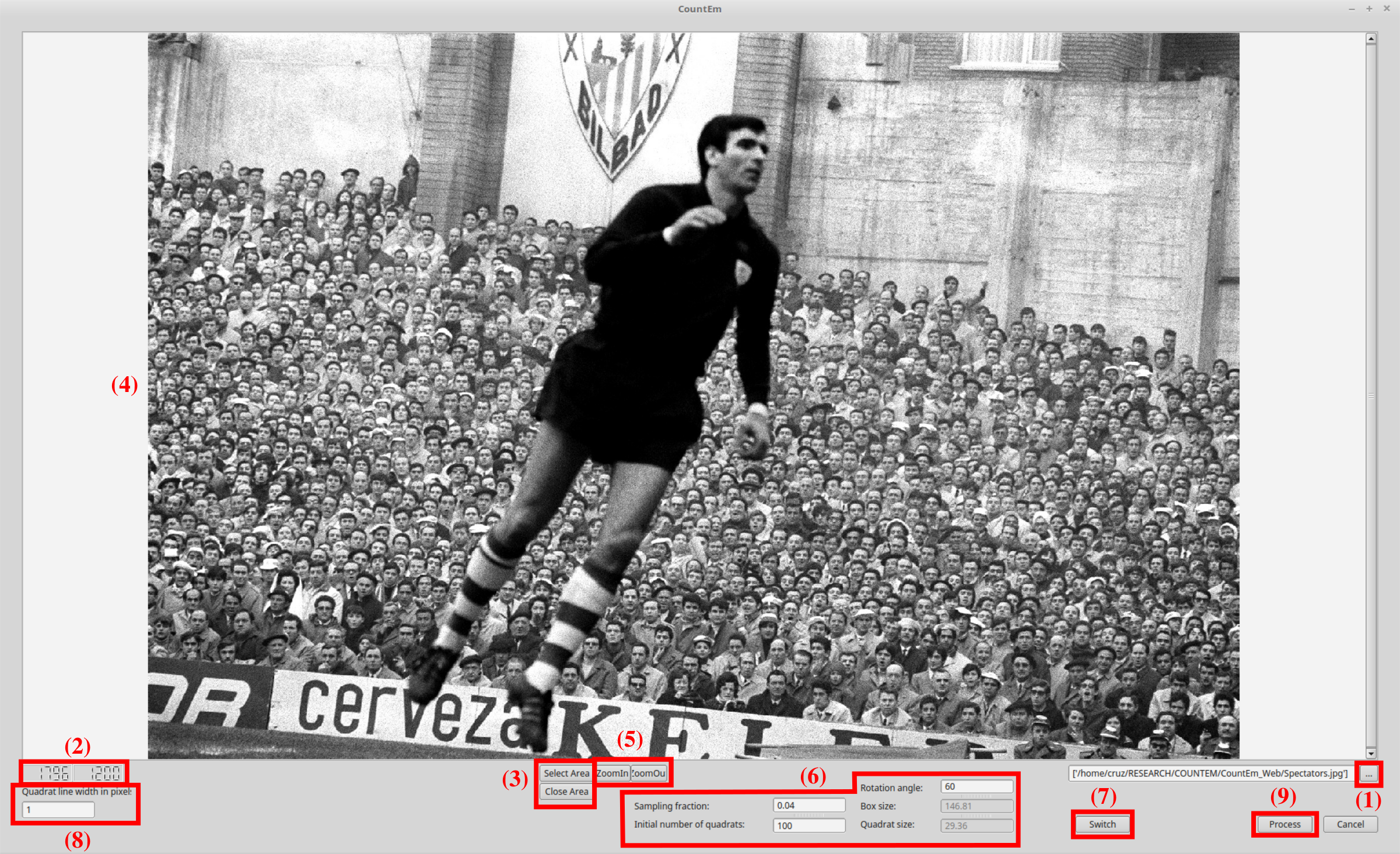
The image size in pixels is displayed in (2).
- (Optional): Click Select Area (3) and create a polygonal region of interest (RoI) by interactively clicking on the image (4). The left (right) mouse button adds (removes) a point. Zoom in and out using (5). The Close Area button (3) draws a line from the last selected point to the initial point and saves the RoI. Multiple RoI's can be defined iteratively.
- Enter the grid parameters in (6):
- Initial number of quadrats: Desired number of quadrats in the whole image (or RoI).
- Sampling fraction: Fraction of the total population that should be sampled.
An alternative grid parametrization can be selected using the Switch button (7):
- Box size: Distance (in pixels) between two consecutive quadrat centres.
- Quadrat size: Side length in pixels of the quadrat (i.e, of the sampling window).
The Rotation angle (Grid rotation angle in degrees) can also be set in (6).
Read our FAQ section in order to choose convenient parameter values.
- Select a convenient Quadrat line width (8) and click Process (9) to generate a uniform random superimposition of the grid of quadrats on the image.
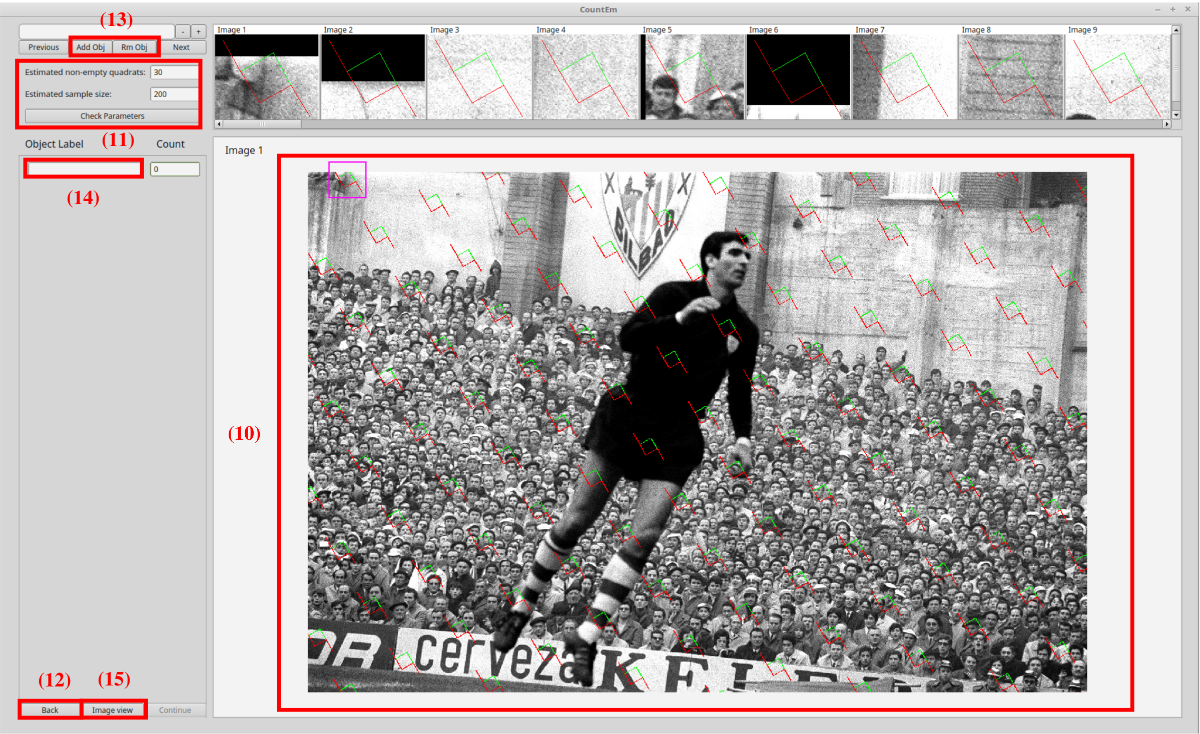
- Visually estimate in (10) the number of non-zero quadrats (should be > 30), and the sample size (should be between 100 and 300). Enter the values in (11). The Check Parameters button will evaluate If the grid is convenient and choose a corrected one if not. The parameters can also be changed by returning to step 4) clicking Back in (12).
- (Optional) Define object labels (for instance different bird species) using Add Obj and Rm Obj (13) to add and remove labels (14).
- Click Image View (15).
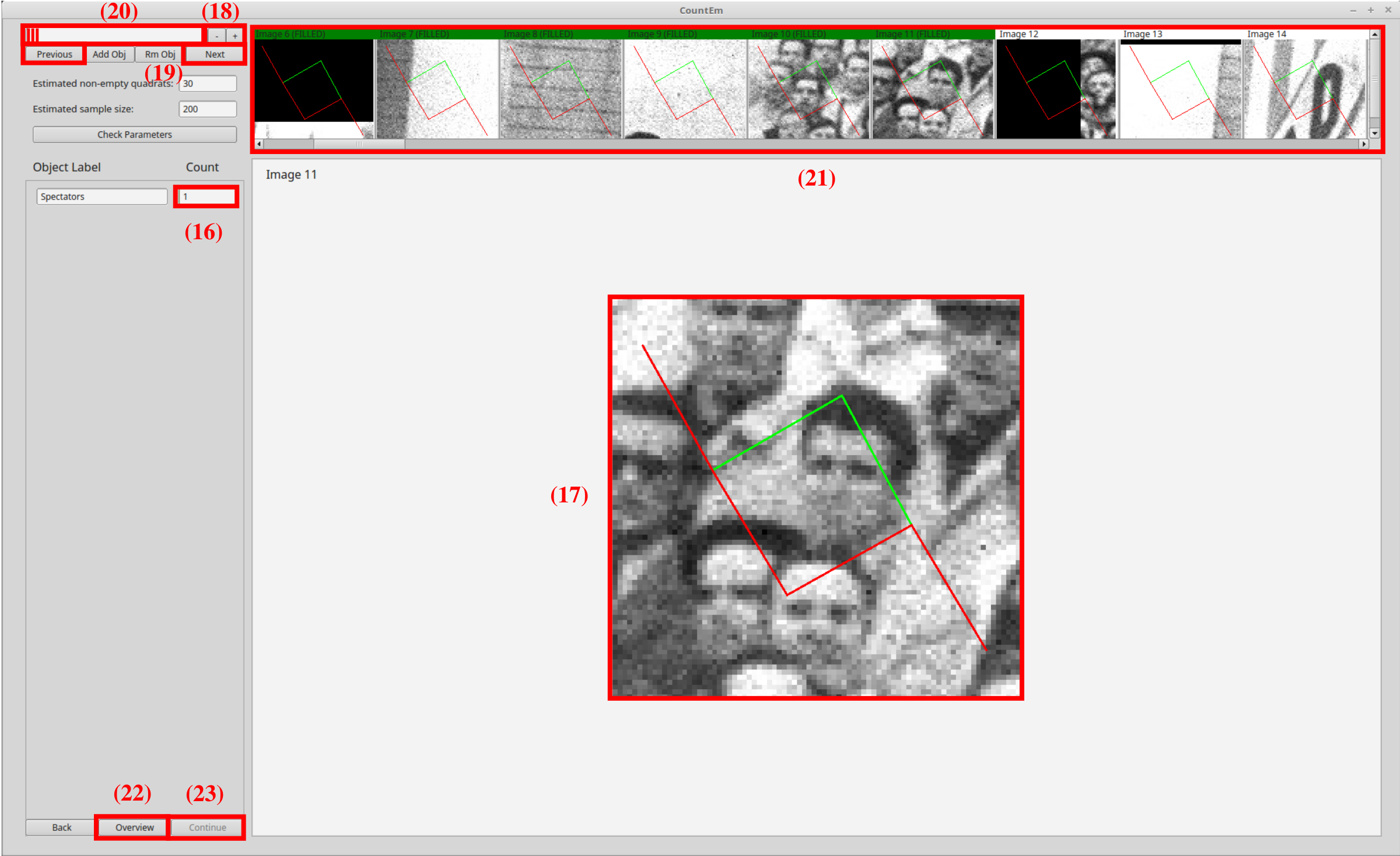
- Enter in (16) the number of particles captured by the magnified quadrat (17).
- A particle is counted in a quadrat only if it has points in common with the quadrat but it does not hit the extended forbidden red line of the quadrat.
- The image can be zoomed in and out using the buttons in (18) or the hotkeys '+' and '-'.
- The previous and next buttons in (19) can be used to switch to the preceding and the following quadrat respectively.
- The number of remaining quadrats can be visualized in the progress bar (20).
- Quadrat selection is also possible by scrolling and clicking interactively in (21).
- The Overview button in (22) shows the grid of quadrats superimposed on the original image (10).
- The active quadrat highlighted with a magenta square in (10).
- After counting the particles in the last quadrat, the progress bar (20) turns green. Click Continue (23).
The results are displayed in the following window :
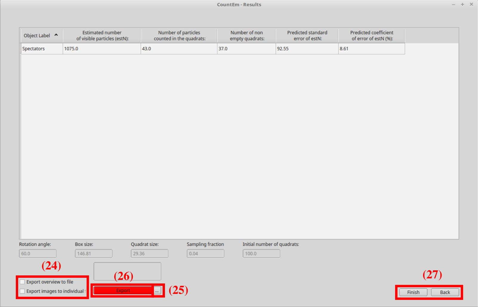
- Estimated number of visible particles (estN): Estimated total number of particles in the image.
- Number of particles counted in the quadrats: Total number of particles captured by the grid of quadrats.
- Number of nonempty quadrats: Total number of quadrats containing at least one particle.
- Predicted standard error of estN: Square root of the predicted error variance of the total number of particles, namely se(estN).
- Predicted coefficient of error of estN (%): Relative standard error in percent, namely 100 * se(estN) / estN = ce(estN) %.
- The numeric results and/or the images can be exported to csv and tiff files respectively by checking the corresponding checkboxes (24). The destination folder can be selected in (25) before clicking the Export button (26), which should turn green.
- Choose to return to step 2), or to finish, in (27).